Overview
Teaching: 30 min
Exercises: 10 minQuestions
What tools are available to easily disseminate our work?
How can we make our work more reproducible?
Objectives
Learn the basics of
RMarkdownandknitrLearn to integrate
Rcode with text and images.
2. Literate programming
- Organize your work
- make work more pleasant for yourself? (less tedium, less manual, less …)
- reduce friction for collaboration?
- reduce friction for communication?
- make your work navigable, interpretable, and repeatable by others?
Getting the analysis right is only one link
Process, packaging, and presentation are often the weak links in the chain.

Markdown
What is Markdown?
Markdownis a particular type of markup language. Markup languages are designed to produce documents from plain text.- You may be familiar with
LaTeX, another (though less human friendly) text markup language. - Tools render markdown to different formats (for example, HTML/pdf/Word).
- The main tool for rendering Markdown is pandoc.
Adapted from Carson Sievert’s markdown slides
Markdown enables fast publication to the web
- Markdown Easy to write and read in an editor.
- HTML Easy to publish and read on web.
Markdown versus HTML code {.code-columns}
This is a Markdown document.

## Medium header <!-- header 2, actually -->

It's easy to do *italics* or __make things bold__.

> All models are wrong, but some are useful. An approximate answer to the right problem is worth a good deal more than an exact answer to an approximate problem.

Code block below. Just affects formatting here.

```
x <- 3 * 4
```

I can haz equations. Inline equations, such as the average is computed as $\frac{1}{n} \sum_{i=1}^{n} x_{i}$. Or display equations like this:


$$
\begin{equation*}
|x|=
\begin{cases} x & \text{if $x\ge 0$,} \\\\
-x &\text{if $x\lt 0$.}
\end{cases}
\end{equation*}
$$


<!DOCTYPE html>
<html>
<head>
<meta http-equiv="Content-Type" content="text/html; charset=utf-8"/>
<title>Title</title>
<!-- MathJax scripts -->
<script type="text/javascript" src="..."></script>
<style type="text/css">
body {
   font-family: Helvetica, arial, sans-serif;
   font-size: 14px;
...
</style>
</head>
<body>
<p>This is a Markdown document.</p>

<h2>Medium header</h2>

<p>It's easy to do <em>italics</em> or <strong>make things bold</strong>.</p>

<blockquote><p>All models are wrong, but some are...</p></blockquote>
<p>Code block below. Just affects formatting here.</p>

<pre><code>x <- 3 * 4
</code></pre>


Markdown versus rendered HTML {.code-columns}
This is a Markdown document.
Medium header
It’s easy to do italics or make things bold.
All models are wrong, but some are useful. An approximate answer to the right problem is worth a good deal more than an exact answer to an approximate problem.
Code block below. Just affects formatting here.
x <- 3 * 4
I can haz equations. Inline equations, such as the average is computed as $\frac{1}{n} \sum_{i=1}^{n} x_{i}$. Or display equations like this:
This is a Markdown document.
Medium header
It’s easy to do italics or make things bold. > All models are wrong, but some are useful. An approximate answer to the right problem is worth a good deal more than an exact answer to an approximate problem. Code block below. Just affects formatting here. x <- 3 * 4 I can haz equations. Inline equations, such as the average is computed as $\frac{1}{n} \sum_{i=1}^{n} x_{i}$. Or display equations like this: $$ \begin{equation*} |
x | = \begin{cases} x & \text{if $x\ge 0$,} \\ -x &\text{if $x\lt 0$.} \end{cases} \end{equation*} $$ |


Markdown can be rendered to multiple formats
pandocis a swiss-army knife tool for conversion`
RMarkdown
RMarkdown is rendered to Markdown {.code-columns}
This is an R Markdown document.
x <- rnorm(1000)
head(x)
## [1] -0.1335833 0.8267038 -1.1034869 -0.6733962 -0.3090355 0.2260558
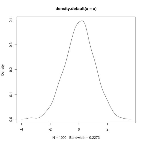
knitr offers a lot of control over representing different types of output. We can also have inline R expressions computed on the fly. The mean $\bar{x} = \frac{1}{n} \sum_{i=1}^{n} x_{i}$ of the 1000 random variates we generated is 0.064. This figure is computed on-the-fly as well. No more copy-paste, including for figures:
plot(density(x))

This is an RMarkdown document.
x <- rnorm(1000)
head(x)
## [1] -0.6759262 -0.6480025 -1.5323815 -0.3424358 0.9884121 1.2100950
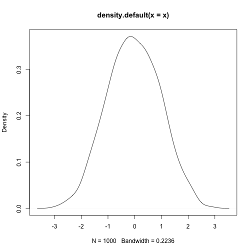
knitr offers a lot of control over representing different types of output. We can also have inline R expressions computed on the fly. The mean $\bar{x} = \frac{1}{n} \sum_{i=1}^{n} x_{i}$ of the 1000 random variates we generated is -0.035. This figure is computed on-the-fly as well. No more copy-paste, including for figures:
plot(density(x))

Ideas, code, and generated results tied together {.code-columns}
This is an RMarkdown document.
x <- rnorm(1000)
head(x)
## [1] -1.0912306 -1.3695738 -0.2707651 -1.2588747 -1.5823117 -1.2076593
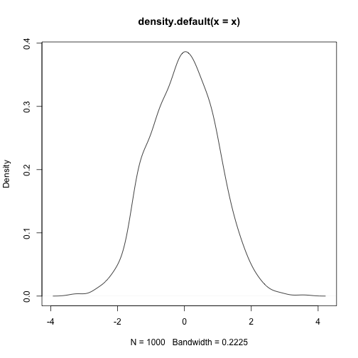
knitr offers a lot of control over representing different types of output. We can also have inline R expressions computed on the fly. The mean $\bar{x} = \frac{1}{n} \sum_{i=1}^{n} x_{i}$ of the 1000 random variates we generated is -0.034. This figure is computed on-the-fly as well. No more copy-paste, including for figures:
plot(density(x))

This is an RMarkdown document. {r} x <- rnorm(1000) head(x) knitr offers a lot of control over representing different types of output. We can also have inline R expressions computed on the fly. The mean $\bar{x} = \frac{1}{n} \sum_{i=1}^{n} x_{i}$ of the 1000 random variates we generated is -0.034. No more copy-paste, including for figures: {r} plot(density(x))
Rendering can be automated is thus repeatable

From within R:
rmarkdown::render("filename.Rmd")
From the command line:
$ Rscript -e "rmarkdown::render('filename.Rmd')"
Summary
RMarkdownenables ideas and questions, the code that implements them, and the results generated by the implementation, to all stay together.RMarkdowntoolchain allows automated, repeatable rendering- for publishing to the web and viewing through a browser
- and (through
LaTeX) to obtain a submittable manuscript (in PDF or Word).
knitris not limited to executingRcode. See the book Dynamic documents withRandknitrby Yihui Xie, part of the CRC Press / Chapman & Hall R Series (2013). ISBN
Key Points
RMarkdownandknitrare powerful tools.Output can be rendered in many formats.
You don’t need to know HTML!